What’s the Deal with Bayesian A/B Testing?

October 24, 2019

David DeFranza

In recent years, Bayesian inference has become increasingly popular among researchers and this interest has begun spilling over into business applications, such as A/B testing. So, what is Bayesian A/B testing? How is it being used? What are the advantages and disadvantages? This blog post will answer these questions.

Given any set of observations, it’s relatively simple to calculate a set of statistics to describe the data. For example, you can calculate a mean which represents the expected value of a given variable in the data, and the variance, which represents the spread of the data.

Imagine you’re examining height: you could measure the heights of 25 individuals, calculate the mean and variance and draw a conclusion about the 25 people you measured.

Unfortunately, when it comes to drawing useful conclusions, it would be better to calculate the mean height of every person in the world. But the only definitive way to do that is to actually measure the height of every single person in the world—a daunting task, if not impossible. So instead, you can use your sample of 25 people to make a generalization about all other people from these observations. This process of generalization is called inference.

The Problem With Inference

Inference presents a few problems which make it an unsettled issue in statistics, science and philosophy.

First, there’s no guarantee that a series of observations captures a true mean value. In other words, if you select 25 people at random from the population of the world, measure their heights and calculate a mean, then repeat this process thousands of times, you’ll likely arrive at different means with every sample.

Similarly, there’s no guarantee you’ll capture the variability in height across the entire population. This variance may be different in every group of 25 you measure, sometimes dramatically so.

All of this means that drawing a reliable, meaningful generalization from a relatively small set of observations remains a challenge.

Frequentist A/B Testing

Given that the true population parameters cannot be measured (e.g., the average height of every person living in the world right now) frequentist inference argues that a measure repeated a sufficient number of times will coalesce around the true measure in the population. This is known as the central limit theorem and is the foundation of frequentist statistics.

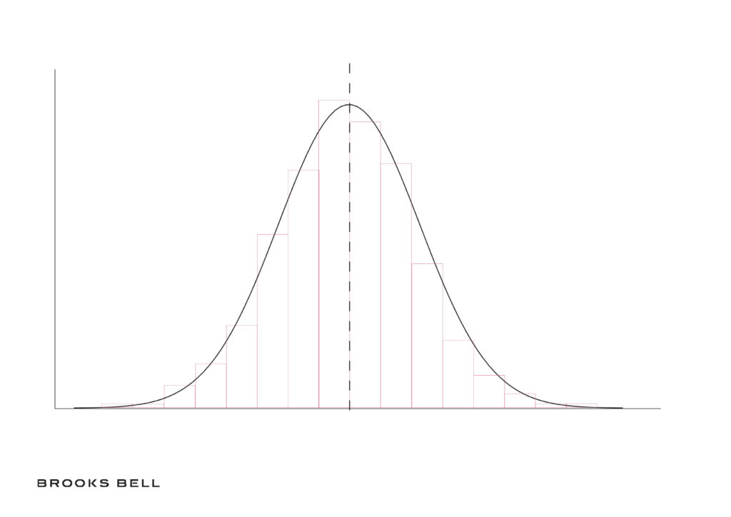
To extend the height example from above, the central limit theorem acknowledges that the mean height of 25 randomly selected individuals will vary from sample to sample, however, these means (and the associated variances) will begin to form a normal curve, with the highest frequency means in the middle with higher and lower values trailing out in both directions with consistent and predictably diminishing frequencies.

Moreover, this curve will be centered on the true population mean. The associated confidence interval (e.g., hypothetically for human height 95% C.I. [160cm, 180cm]) tells you that if your measurements were repeated many more times, you’d expect 95 percent of the resulting means to fall within the limits of the provided interval. This is verified through the use of a statistical test, like a T-test, or through a simulation like bootstrapping or permutation tests.

Essentially, this tells you what your expectation of the mean and the associated variance around this expectation will be. Then, you can evaluate subsequent observations in relation to this expectation.

Inference becomes important to A/B testing when comparing the observed outcome of one test variation to another. Essentially, you’re hoping to compare the mean of an outcome variable (e.g., sales or sign-ups) in two different populations. One population is the control. The second population is the challenger.

Given a reasonably large sample drawn randomly from both populations, you can compare the overlap of their distributions. This determines whether the likelihood an observed difference was a true difference, or simply the result of chance. This provides a conservative assessment of, for example, the probability that customers experiencing a new variation will complete a purchase is higher than customers in the control experience.

But the frequentist model ushers in some of the reasons website analysts have turned to Bayesian A/B tests: it requires precise decisions about the total sample size, it cannot be evaluated as data is being collected, and the conclusion offers only a binary “yes” or “no” – it doesn’t provide additional guidance about how to interpret lack of significance.

Bayesian A/B Testing

The fundamental difference between frequentist and Bayesian inference is that while frequentist inference relies on a series of independent observations, Bayesian inference acknowledges that each new observation should be understood in the context of previous observations.

In other words, if you measure a person’s height to be 170cm, you should use this to make inferences about height generally in relation to previous measures of height. The previous measures of height, in this example are referred to as the prior and the resulting inference about heights after we consider the latest measurement is the posterior.

We can illustrate the idea of conditionality with a simple example:

Imagine there are two bowls of candies. The first bowl contains 30 red candies and 10 blue candies. The second bowl contains 20 of each candy. Suppose you pick a candy, without looking, from one of the bowls at random and the candy is red. What is the probability the candy came from the first bowl?

This is an illustration of the conditional probability p(bowl one | red) or, the probability of bowl 1 given a drawn red candy. Bayes’ theorem provides a means of calculating this probability:

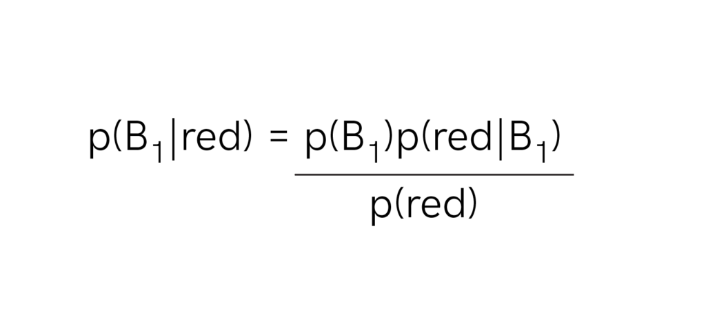
where p(B₁) is the probability of picking from bowl one, which we know is ½, p(red | B₁) is the probability of picking a red candy in from bowl one, which we know is ¾, and p(red) is the probability of picking a red candy in general, which we know is 5/8.

Thus:

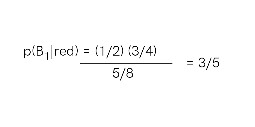
In this case, p(B₁) is an example of the prior probability, p(red|B₁) is an example of the likelihood, p(red) is an example of the evidence, and p(bowl one | red) is the posterior probability.

In practice, the prior probability can be based on informative observations, the average conversion rate for your website over the last 12 months, for example, subjective knowledge such as a manager’s belief about the demographics of a customer base, or taken as uninformed, such as when all possible outcomes are given equal probability.

Bayesian A/B Testing

Just as in the frequentist case, we’re primarily interested in whether a new design to a website performs better than the existing, control design. Calculating the difference between two variations isn’t as easy as calculating a simple conditional probability. As such, I’ll walk through the algorithm for conducting a Bayesian A/B test, but not the steps to calculating a solution analytically.

Importantly, the important metrics and parameters can be calculated both analytically and numerically–most commonly with Markov Chain Monte Carlo (MCMC) estimation.

Here’s the basic algorithm:

Determine a prior based on historical data or managerial knowledge
Determine the desired lift (e.g., 10 percent) and desired error rate (acceptable chance a winning variation could, in fact, be a losing variation)
Assign the control and variation(s) the previously determined prior (in practice, the control is typically assigned the strong prior determined from historical data and variations are assigned an uninformed prior based on a uniform distribution)
Launch the test, splitting samples evenly into each test group.
Regularly (or continuously) measure the number of individuals in and the outcome metric (e.g. conversion rate) for each test group.
Regularly (or continuously) calculated the expected loss of each variation. Once one variation’s expected loss drops below the predetermined error rate, end the test and declare that variation the winner.

Note the important differences in this process.

First, unlike frequentist methods, no sample size is declared prior to starting the test. Second, there’s no problem with regularly checking the results; in fact, regularly checking the results is part of the process. Also, note that the control typically receives a stronger prior than the challenging variations. This means that Bayesian A/B testing is sensitive to any difference that may exist, regardless of how small it is.

Bayesian A/B testing enables you to find a difference between variations even with relatively small sample sizes. It also allows for constant monitoring, which means tests can more reasonably be called if all challenging variations appear to be underperforming. Finally, because of the continuous or regular updates and use of prior information, Bayesian tests can reach a conclusion much faster.

However, there are also significant drawbacks. Deriving a solution is computationally intensive and, unlike most frequentist methods, relies on complex calculus to determine the constrained optimization solution (if solved analytically) or equally complex simulation methods (e.g., MCMC) if numerical solutions are derived. Though some testing tools, like Optimizely, are implementing Bayesian methods, understanding and explaining these methods is much more complex, though the results can sometimes be more intuitive.

Ultimately, implementing Bayesian A/B testing requires a lengthy, technical discussion involving a considerable amount of math. As Bayesian approaches to A/B testing becomes more popular, you can use this new understanding to determine whether this approach is appropriate and how to interpret the results.